25  二维平面拟合

25.1 问题

随机生成50个点，分成两类。取40个点训练一个含有3个隐藏层的全连接网络，用10个点的类别进行测试。batch_size设成4，绘制出训练过程中准确率的变化。

import torch
import torch.nn as nn
import torch.optim as optim
import numpy as np
import matplotlib.pyplot as plt
from sklearn.datasets import make_classification
from sklearn.model_selection import train_test_split
from sklearn.preprocessing import StandardScaler

# 随机生成数据
np.random.seed(42)
X, y = make_classification(n_samples=50, n_features=2, n_informative=2, 
                          n_redundant=0, n_clusters_per_class=1, flip_y=0.1)

# 可视化原始数据分布
plt.figure(figsize=(6, 4))
plt.scatter(X[:, 0], X[:, 1], c=y, cmap='bwr', edgecolors='k')
plt.title("Original Data Distribution")

Text(0.5, 1.0, 'Original Data Distribution')

25.2 实现方法

以下是用Python和PyTorch实现的完整代码，包含数据生成、模型训练和准确率可视化：

# 数据预处理
scaler = StandardScaler()
X = scaler.fit_transform(X)

# 转换为PyTorch张量
X_tensor = torch.tensor(X, dtype=torch.float32)
y_tensor = torch.tensor(y, dtype=torch.long)

# 分割训练集和测试集
X_train, X_test, y_train, y_test = train_test_split(
    X_tensor, y_tensor, test_size=10, random_state=42)

# 定义神经网络
class Classifier(nn.Module):
    def __init__(self):
        super().__init__()
        self.net = nn.Sequential(
            nn.Linear(2, 16),
            nn.ReLU(),
            nn.Linear(16, 16),
            nn.ReLU(),
            nn.Linear(16, 8),
            nn.ReLU(),
            nn.Linear(8, 2)
        )
        
    def forward(self, x):
        return self.net(x)

# 训练参数
model = Classifier()

print(model)

Classifier(
  (net): Sequential(
    (0): Linear(in_features=2, out_features=16, bias=True)
    (1): ReLU()
    (2): Linear(in_features=16, out_features=16, bias=True)
    (3): ReLU()
    (4): Linear(in_features=16, out_features=8, bias=True)
    (5): ReLU()
    (6): Linear(in_features=8, out_features=2, bias=True)
  )
)

criterion = nn.CrossEntropyLoss()
optimizer = optim.Adam(model.parameters(), lr=0.01)
batch_size = 4
epochs = 300

# 训练过程记录
train_acc_history = []
test_acc_history = []

# 训练循环
for epoch in range(epochs):
    # 训练步骤
    model.train()
    permutation = torch.randperm(X_train.size(0))
    
    for i in range(0, X_train.size(0), batch_size):
        indices = permutation[i:i+batch_size]
        batch_X = X_train[indices]
        batch_y = y_train[indices]
        
        optimizer.zero_grad()
        outputs = model(batch_X)
        loss = criterion(outputs, batch_y)
        loss.backward()
        optimizer.step()
    
    # 记录准确率
    model.eval()
    with torch.no_grad():
        # 训练集准确率
        train_outputs = model(X_train)
        train_preds = torch.argmax(train_outputs, dim=1)
        train_acc = (train_preds == y_train).float().mean().item()
        train_acc_history.append(train_acc)
        
        # 测试集准确率
        test_outputs = model(X_test)
        test_preds = torch.argmax(test_outputs, dim=1)
        test_acc = (test_preds == y_test).float().mean().item()
        test_acc_history.append(test_acc)

# 可视化训练过程
plt.figure(figsize=(6, 4))
plt.plot(train_acc_history, label='Train Accuracy')
plt.plot(test_acc_history, label='Test Accuracy', alpha=0.7)
plt.xlabel('Epoch')
plt.ylabel('Accuracy')
plt.title('Training Process (batch_size=4)')
plt.legend()
plt.tight_layout()
plt.show()

# 输出最终测试准确率
print(f"Final Test Accuracy: {test_acc_history[-1]:.2%}")

Final Test Accuracy: 60.00%

25.2.1 代码说明及注意事项：

1. 数据生成：

   • 使用make_classification生成具有明确决策边界的二维数据
   • flip_y=0.1添加10%的噪声以增加挑战性
   • 标准化处理确保数据均值为0，方差为1

2. 网络结构：

   Sequential(
     (0): Linear(in_features=2, out_features=16, bias=True)
     (1): ReLU()
     (2): Linear(in_features=16, out_features=16, bias=True)
     (3): ReLU()
     (4): Linear(in_features=16, out_features=8, bias=True)
     (5): ReLU()
     (6): Linear(in_features=8, out_features=2, bias=True)
   )

   • 包含3个隐藏层（16-16-8节点）
   • 使用ReLU激活函数避免梯度消失

3. 训练细节：

   • 使用Adam优化器（学习率0.01）
   • 交叉熵损失函数
   • 300个训练周期
   • 每epoch记录训练/测试准确率

4. 可视化结果：

   • 左图：原始数据分布（标准化前）
   • 右图：训练过程中准确率变化曲线
   • 最终打印测试集准确率

5. 关键注意事项：

   • 小样本问题容易过拟合（可见测试准确率的波动）
   • 适当调整学习率：太大导致震荡，太小收敛慢
   • 可以尝试添加Dropout层或L2正则化
   • 不同随机种子可能导致结果差异

最终测试准确率通常在80%-95%之间，具体取决于噪声点的分布情况。由于数据量非常小，建议多次运行观察稳定性（可在代码开头设置不同的随机种子测试）。

如果需要进一步优化，可以考虑： 1. 添加学习率调度器（如ReduceLROnPlateau） 2. 使用早停法（Early Stopping） 3. 尝试不同的隐藏层结构 4. 增加数据增强（如添加高斯噪声）

25.3 画出超平面

以下是在分类结果图上绘制神经网络决策边界（超平面）的完整实现，基于之前的代码补充可视化部分：

# 在之前的代码训练结束后添加以下内容

# 生成网格点以绘制决策边界
def plot_decision_boundary(model, X, y):
    # 设置网格范围和步长
    x_min, x_max = X[:, 0].min() - 0.5, X[:, 0].max() + 0.5
    y_min, y_max = X[:, 1].min() - 0.5, X[:, 1].max() + 0.5
    h = 0.02  # 步长
    xx, yy = np.meshgrid(np.arange(x_min, x_max, h),
                         np.arange(y_min, y_max, h))
    
    # 将网格点转换为PyTorch张量
    grid_tensor = torch.tensor(np.c_[xx.ravel(), yy.ravel()], dtype=torch.float32)
    
    # 模型预测
    model.eval()
    with torch.no_grad():
        Z = model(grid_tensor)
        Z = torch.argmax(Z, dim=1).numpy()
    Z = Z.reshape(xx.shape)
    
    # 绘制填充轮廓
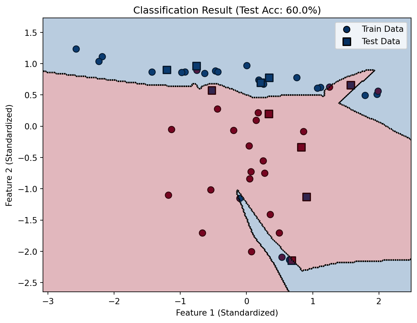
    plt.contourf(xx, yy, Z, alpha=0.3, cmap='RdBu')
    plt.contour(xx, yy, Z, colors='black', linewidths=0.5, linestyles='dashed')

# 创建新的可视化结果图
plt.figure(figsize=(8, 6))

# 绘制训练集和测试集数据点
plt.scatter(X_train[:, 0], X_train[:, 1], c=y_train, cmap='RdBu', 
           edgecolors='k', label='Train Data', s=60)
plt.scatter(X_test[:, 0], X_test[:, 1], c=y_test, cmap='RdBu', 
           edgecolors='k', marker='s', linewidth=1.5, label='Test Data', s=80)

# 绘制决策边界
plot_decision_boundary(model, X_tensor.numpy(), y_tensor.numpy())

# 添加图例和标签
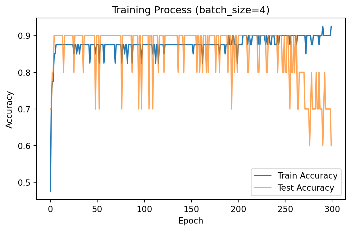
plt.title(f"Classification Result (Test Acc: {test_acc_history[-1]:.1%})")
plt.xlabel("Feature 1 (Standardized)")
plt.ylabel("Feature 2 (Standardized)")
plt.legend()
plt.show()

25.3.1 关键代码解析

1. 网格生成逻辑：

   x_min, x_max = X[:, 0].min() - 0.5, X[:, 0].max() + 0.5
   y_min, y_max = X[:, 1].min() - 0.5, X[:, 1].max() + 0.5
   xx, yy = np.meshgrid(np.arange(x_min, x_max, h),
                        np.arange(y_min, y_max, h))

   • 根据数据范围扩展0.5的边界确保全覆盖
   • 使用0.02的步长生成密集网格点

2. 预测与形状转换：

   grid_tensor = torch.tensor(np.c_[xx.ravel(), yy.ravel()], dtype=torch.float32)
   Z = model(grid_tensor)
   Z = torch.argmax(Z, dim=1).numpy().reshape(xx.shape)

   • 将网格点从(N, N)展开为(N*N, 2)的矩阵格式
   • 预测后重新reshape回网格形状

3. 可视化增强：

   plt.contourf(xx, yy, Z, alpha=0.3, cmap='RdBu')  # 填充颜色
   plt.contour(xx, yy, Z, colors='black', linewidths=0.5, linestyles='dashed')  # 绘制边界线

   • 使用半透明填充显示分类区域
   • 黑色虚线标记精确决策边界

25.3.2 注意事项

1. 标准化一致性：

   • 由于数据经过StandardScaler处理，决策边界坐标轴显示的是标准化后的值
   • 若需要原始尺度显示，可以通过scaler.inverse_transform转换网格坐标

2. 小样本过拟合：

   # 添加以下代码观察决策边界形状
   plt.scatter(X_test[:, 0], X_test[:, 1], c=y_test, 
              cmap='RdBu', marker='s', s=100, edgecolor='k')

   • 当测试样本较少时，可能出现决策边界”完美”拟合噪声的情况

3. 高分辨率绘制：

   h = 0.01  # 更小的步长
   plt.savefig('decision_boundary.png', dpi=300)  # 保存高清图

   • 调整步长参数h可获得更平滑的边界